Demonstration of AMP for SMLR
This example shows how to use GAMP for multiclass linear classification via multinomial logistic regression. SPA-SHyGAMP and MSA-SHyGAMP can be invoked using the "mcGAMP" function.
Contents
Data generation
For this example, the data is generated as follows:
1.) 
 -ary class labels are drawn uniformly, i.e.
  .
.
2.) The set of class means  , each in
  , are drawn mutually orthogonal,
  -sparse, have uniform support, and each has norm
  . This is achieved by zero-padding the columns of the left singular vectors of a
  Gaussian random matrix, and then scaling by
  .
.
3.) The feature variance  is set in order for the data to have a desired Bayes error rate, and is a function of
  and
and  .
.
4.) Finally, each feature vector  .
.
We note two things:
1.) This data model is matched to the multinomial logistic activation function.
2.) For a given weight matrix  , the test-error-rate can be computed using a procedure that involves MATLAB's
  command (see eq. (82)-(83) in the paper for details).
% data parameters
N = 30000;     % number of features
M = 300;       % number of training samples
K = 30;        % number of discriminatory features
D = 4;         % number of classes
Pbayes = .15;  % Bayes error rate

[y_train, A_train, mu, v] = buildDatasets(D,M,N,K,Pbayes);

% A_train is an M x N matrix, where each row is a training feature vector.
% y_train is an M x 1 vector, where each element is the class label
% corresponding to a row of A_train.
% mu is an N x D matrix, where each column is the mean of the D'th class.
% v is the cloud variance.

xBayes = mu; % Bayes optimal classifier
SPA-SHyGAMP
% SPA-SHyGAMP finds an approximation to the probability or error minimizing
% classifier.


% the function mcGAMP runs SPA-SHyGAMP by defualt.
% calling mcGAMP with only y and A as input arguments uses the default
% algorithm parameters.  Optionally, one can use
% mcGAMP(y,A,opt_mc,opt_gamp), where opt_mc = MCOpt() and opt_gamp is a
% structure of gamp options.  Note that the default GAMP options in mcGAMP
% (eg the stepsize) are not the same as the default GAMP options.
estFin = mcGAMP(y_train,A_train);

% evaluate test-error-rate
test_error_SPA = testErrorRate(estFin.xhat, mu, v);

fprintf('SPA-SHyGAMP test error rate is %.3f\n',test_error_SPA)

% rerun SPA-SHyGAMP, but with plots on
opt_mc = MCOpt();
opt_mc.plot_hist = 1; % number indicates figure number
opt_mc.plot_wgt = 2;

% must also specify model in order to compute error within mcGAMP
opt_mc.x_bayes = mu;
opt_mc.mu = mu;
opt_mc.v = v;
opt_mc.Pbayes = Pbayes;

% call mcGAMP, now with the structure opt_mc as the thrid input
mcGAMP(y_train, A_train, opt_mc);
************************************************************************

beginning SPA-SHyGAMP

SPA-SHyGAMP finished.
Runtime = 6.45 seconds.
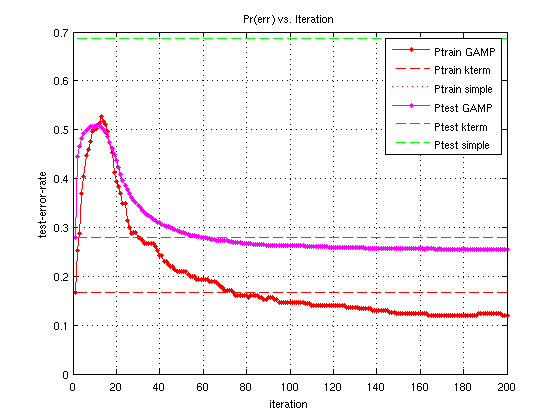
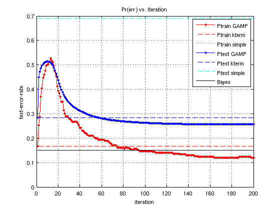
Training-error-rate = 0.120
SPA-SHyGAMP test error rate is 0.256


************************************************************************

beginning SPA-SHyGAMP
Known theoretical error function

SPA-SHyGAMP finished.
Runtime = 6.73 seconds.
Training-error-rate = 0.120
Test-error-rate (theo) = 0.256
Plot descriptions
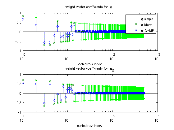
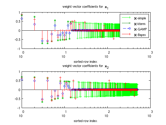
The first set of plots show the first 500 elements of selected weight vectors, with their indices ordered according to the sorted order of the absolute values of  -simple. Quick descriptions of the weight vectors are:
1.)  -simple is the class-conditional empirical mean of
  . In other words,
  , where
  is the number of training examples in class
  .
.
2.)  -kterm is
  -simple where the
  largest elements (by absolute value) of each column are retained, with the remaining set to zero.
  is chosen based on
  ,
,  , and
, and  , and is an estimate for the largest number of elements in
  that can be accurately learned (for details, see pg. 46 in the thesis).
3.)  -GAMP is the weight matrix returned by GAMP.
4.)  -Bayes is the Bayes optimal weight matrix.
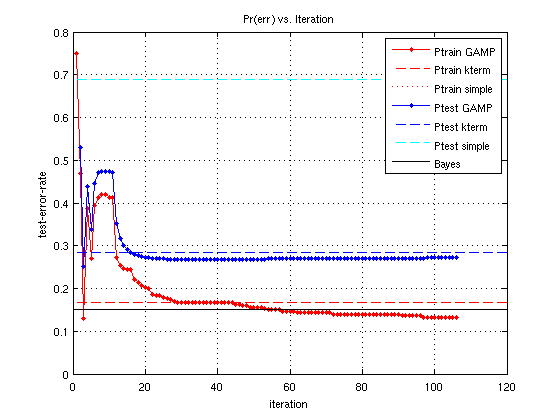
The second plot shows the test-error-rate and the training-error-rate vs GAMP iteration for the various weight matrices shown in the first plot (although, note  -GAMP changes with each GAMP iteration, and values plotted in the first figure are the final values of
  -GAMP).
MSA-SHyGAMP
% MSA-SHyGAMP solves the traditional ell_1 regularized objective.

opt_mc = MCOpt();
opt_mc.SPA = false; % set this option to false to run MSA-SHyGAMP
estFin = mcGAMP(y_train,A_train,opt_mc);

% evaluate test-error-rate
test_error_MSA = testErrorRate(estFin.xhat, mu, v);

fprintf('MSA-SHyGAMP test error rate is %.3f\n',test_error_MSA)

% rerun SPA-SHyGAMP with plots on
opt_mc = MCOpt();
opt_mc.SPA = false;
opt_mc.plot_hist = 3;
opt_mc.plot_wgt = 4;
opt_mc.x_bayes = mu;
opt_mc.mu = mu;
opt_mc.v = v;
opt_mc.Pbayes = Pbayes;

mcGAMP(y_train, A_train, opt_mc);
************************************************************************

beginning MSA-SHyGAMP

MSA-SHyGAMP finished.
Runtime = 10.32 seconds.
Training-error-rate = 0.133
MSA-SHyGAMP test error rate is 0.272


************************************************************************

beginning MSA-SHyGAMP
Known theoretical error function

MSA-SHyGAMP finished.
Runtime = 10.94 seconds.
Training-error-rate = 0.133
Test-error-rate (theo) = 0.272

SPA-SHyGAMP with emprical test data
% Now we will demonstrate using mcGAMP with empirical test data.

% first, generate test data
M_test = 1e4;
A_test = repmat(mu,1,ceil(M_test/D));
A_test = A_test(:,1:M_test)' + sqrt(v) * randn(M_test,N);
y_test = repmat(1:D,1,ceil(M_test/D));
y_test = y_test(1:M_test)';

opt_mc = MCOpt();
opt_mc.plot_hist = 5;
opt_mc.plot_wgt = 6;
opt_mc.A_test = A_test; % put the test features in opt_mc.A_test
opt_mc.y_test = y_test; % put the test features in opt_mc.y_test

mcGAMP(y_train, A_train, opt_mc);
************************************************************************

beginning SPA-SHyGAMP
Known empirical error function

SPA-SHyGAMP finished.
Runtime = 7.33 seconds.
Training-error-rate = 0.120
Test-error-rate (emp) = 0.255
