Contents

%Jason T. Parker
%31 Oct 2013
%This is a simple example to illustrate Matrix Completion using BiG-AMP.
%This code is a simplified version of trial_matrixCompletion. Some of the
%options are set differently for simplicity.

Clean Slate

clear all
clc

%Add paths for matrix completion
setup_MC

Generate the Unknown Low Rank Matrix

%Firt, we generate some raw data. The matrix will be MxL with rank N
M = 500;
L = 500;
N = 4;

%Generate the two matrix factors, recalling the data model Z = AX
A = randn(M,N);
X = randn(N,L);

%Noise free signal
Z = A*X;

%Define the error function for computing normalized mean square error.
%BiG-AMP will use this function to compute NMSE for each iteration
error_function = @(qval) 20*log10(norm(qval - Z,'fro') / norm(Z,'fro'));

AWGN Noise

%We will corrupt the observations of Z, denoted Y, with AWGN. We will
%choose the noise variance to achieve an SNR (in dB) of
SNR = 50;

%Determine the noise variance that is consistent with this SNR
nuw = norm(reshape(Z,[],1))^2/M/L*10^(-SNR/10);

%Generate noisy data
Y = Z + sqrt(nuw)*randn(size(Z));

Observe a fraction of the noisy matrix entries

%For matrix completion, we observe only a fraction of the entries of Y. We
%denote this fraction as p1
p1 = 0.3;


%Choose a fraction p1 of the entries to keep. Omega is an MxL matrix of
%logicals that will store these locations
omega = false(M,L);
ind = randperm(M*L);
omega(ind(1:ceil(p1*M*L))) = true;

%Set the unobserved entries of Y to zero
Y(~omega) = 0;

Define options for BiG-AMP

%Set options
opt = BiGAMPOpt; %initialize the options object with defaults

%Use sparse mode for low sampling rates
if p1 <= 0.2
    opt.sparseMode = 1;
end

%Provide BiG-AMP the error function for plotting NMSE
opt.error_function = error_function;

%Specify the problem setup for BiG-AMP, including the matrix dimensions and
%sampling locations. Notice that the rank N can be learned by the EM code
%and does not need to be provided in that case. We set it here for use by
%the low-level codes which assume a known rank
problem = BiGAMPProblem();
problem.M = M;
problem.N = N;
problem.L = L;
[problem.rowLocations,problem.columnLocations] = find(omega);

Specify Prior objects for BiG-AMP

%Note: The user does not need to build these objects when using EM-BiG-AMP,
%as seen below.

%First, we will run BiG-AMP with knowledge of the true distributions. To do
%this, we create objects that represent the priors and assumed log
%likelihood

%Prior distribution on X is Gaussian. The arguments are the mean and variance.
%Notice that we can use a scalar estimator that will be applied to each
%component of the matrix.
gX = AwgnEstimIn(0, 1);

%Prior on A is also Gaussian
gA = AwgnEstimIn(0, 1);


%Log likelihood is Gaussian, i.e. we are considering AWGN
if opt.sparseMode
    %In sparse mode, only the observed entries are stored
    gOut = AwgnEstimOut(reshape(Y(omega),1,[]), nuw);
else
    gOut = AwgnEstimOut(Y, nuw);
end

Run BiG-AMP

%Initialize results as empty. This struct will store the results for each
%algorithm
results = [];

%Run BiGAMP
disp('Starting BiG-AMP')
tstart = tic;
[estFin,~,estHist] = ...
    BiGAMP(gX, gA, gOut, problem, opt); %#ok<*ASGLU>
tGAMP = toc(tstart);


%Save results for ease of plotting
loc = length(results) + 1;
results{loc}.name = 'BiG-AMP'; %#ok<*AGROW>
results{loc}.err = estHist.errZ(end);
results{loc}.time = tGAMP;
results{loc}.errHist = estHist.errZ;
results{loc}.timeHist = estHist.timing;

Starting BiG-AMP

Run EM-BiG-AMP

%Now we run EM-BiG-AMP. Notice that EM-BiG-AMP requires only the
%observations Y, the problem object, and (optional) options. The channel
%objects are not provided. EM-BiG-AMP learns these parameters, including
%the noise level.
disp('Starting EM-BiG-AMP')
disp(['The true value of nuw was ' num2str(nuw)])
%Run BGAMP
tstart = tic;
[estFin,~,~,estHist] = ...
    EMBiGAMP_MC(Y,problem,opt);
tGAMP = toc(tstart);


%Save results
loc = length(results) + 1;
results{loc}.name = 'EM-BiG-AMP'; %#ok<*AGROW>
results{loc}.err = opt.error_function(estFin.Ahat*estFin.xhat);
results{loc}.time = tGAMP;
results{loc}.errHist = estHist.errZ;
results{loc}.timeHist = estHist.timing;

Starting EM-BiG-AMP
The true value of nuw was 3.9111e-05
It 0001 nuX = 9.676e-01 meanX = 0.000e+00 tol = 1.000e-04 nuw = 3.870e-02 SNR = 20.00 Error = -57.1047 numIt = 0030
It 0002 nuX = 1.629e-01 meanX = 0.000e+00 tol = 1.070e-05 nuw = 4.174e-05 SNR = 49.71 Error = -62.5965 numIt = 0030
It 0003 nuX = 1.631e-01 meanX = 0.000e+00 tol = 9.437e-06 nuw = 3.689e-05 SNR = 50.25 Error = -62.5963 numIt = 0031
It 0004 nuX = 1.631e-01 meanX = 0.000e+00 tol = 9.437e-06 nuw = 3.887e-05 SNR = 50.25 Error = -62.5967 numIt = 0031

Run EM-BiG-AMP with rank learning using rank contraction

%EM-BiG-AMP offers two options for rank learning with matrix completion.
%The first option starts with an over-estimate for the rank and looks for a
%large gap in the singular values of the estiamted X matrix. When a gap
%develops, EM-BiG-AMP truncates the rank to this value. This approach works
%well when the true matrix Z has a distinct gap in its singular values.
%This approach is also generally faster.

%Turn on rank learning using rank contraction. Note that this is option 2
%for learnRank. In this mode, the initial rank will be selected as the
%maximum rank such that a rank N matrix that is MxL can be determined
%uniquely from the number of provided measurements. (This is based on the
%degrees of freedom in the SVD of such a matrix.)

%We can enable this rank learning mode by setting
%EMopt.learnRank = 2;
%However, this is currently the default when no rank is specified in the
%problem setup, so we can simply set
problem.N = [];

disp('Starting EM-BiG-AMP with rank contraction')
disp(['Note that the true rank was ' num2str(N)])
%Run BGAMP
tstart = tic;
[estFin,~,~,estHist] = ...
    EMBiGAMP_MC(Y,problem,opt);
tGAMP = toc(tstart);



%Save results
loc = length(results) + 1;
results{loc}.name = 'EM-BiG-AMP (Rank Contraction)'; %#ok<*AGROW>
results{loc}.err = error_function(estFin.Ahat*estFin.xhat);
results{loc}.time = tGAMP;
results{loc}.errHist = estHist.errZ;
results{loc}.timeHist = estHist.timing;
results{loc}.rank = size(estFin.xhat,1);

Starting EM-BiG-AMP with rank contraction
Note that the true rank was 4
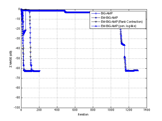
It 0001 nuX = 4.778e-02 meanX = 0.000e+00 tol = 1.000e-04 nuw = 3.870e-02 SNR = 20.00 Error = -21.5452 numIt = 0050
Updating rank estimate from 81 to 4 on iteration 1
It 0002 nuX = 4.457e-02 meanX = 0.000e+00 tol = 1.000e-04 nuw = 2.481e-02 SNR = 21.28 Error = -57.5846 numIt = 0062
It 0003 nuX = 2.154e-01 meanX = 0.000e+00 tol = 1.048e-05 nuw = 4.088e-05 SNR = 49.80 Error = -62.5965 numIt = 0030
It 0004 nuX = 2.156e-01 meanX = 0.000e+00 tol = 9.437e-06 nuw = 3.689e-05 SNR = 50.25 Error = -62.5964 numIt = 0031
It 0005 nuX = 2.156e-01 meanX = 0.000e+00 tol = 9.437e-06 nuw = 3.887e-05 SNR = 50.25 Error = -62.5967 numIt = 0031

Run EM-BiG-AMP with rank learning using penalized log-likelihood maximization

%The second option for rank learning starts with a small rank and gradually
%increases the rank. At each tested rank, we evalute the AICc criteria.
%When this criteria stops improving, we take the rank corresponding to the
%best value of AICc as our rank estimate.

%This approach is tuned fairly conservatively to ensure good performance.
%It works well on noisy data and problems where the singular values tail
%off slowly without a clear-cut rank. However, this approach is generally
%slower than the rank contraction method.


%We limit the number of iterations that BiG-AMP is allowed during each
%EM iteration to reduce run time
opt.nit = 250; %limit iterations

%We also override a few of the default EM options. Options that we do not
%specify will use their defaults
EMopt.maxEMiter = 200; %This is the total number of EM iterations allowed
EMopt.maxEMiterInner = 5; %This is the number of EM iterations allowed for each rank guess
EMopt.learnRank = 1; %The AICc method is option 1
%EMopt.rankStart = 1; This is the default. can be changed if desired.
%   should be less than the true rank


disp('Starting EM-BiG-AMP with rank learning using penalized log-likelihood maximization')
disp(['Note that the true rank was ' num2str(N)])
%Run BGAMP
tstart = tic;
[estFin,~,~,estHist] = ...
    EMBiGAMP_MC(Y,problem,opt,EMopt);
tGAMP = toc(tstart);


%Save results
loc = length(results) + 1;
results{loc}.name = 'EM-BiG-AMP (pen. log-like)'; %#ok<*AGROW>
results{loc}.err = error_function(estFin.Ahat*estFin.xhat);
results{loc}.time = tGAMP;
results{loc}.errHist = estHist.errZ;
results{loc}.timeHist = estHist.timing;
results{loc}.rank = size(estFin.xhat,1);

Starting EM-BiG-AMP with rank learning using penalized log-likelihood maximization
Note that the true rank was 4
It 0001 nuX = 3.870e+00 meanX = 0.000e+00 tol = 1.000e-04 nuw = 3.870e-02 SNR = 20.00 Error = -1.4718 numIt = 0250
It 0002 nuX = 1.299e-01 meanX = 0.000e+00 tol = 1.000e-04 nuw = 2.743e+00 SNR = -3.73 Error = -1.4684 numIt = 0115
It 0003 nuX = 3.393e-01 meanX = 0.000e+00 tol = 1.000e-04 nuw = 2.748e+00 SNR = -4.29 Error = -1.4702 numIt = 0047
It 0004 nuX = 4.685e-01 meanX = 0.000e+00 tol = 1.000e-04 nuw = 2.746e+00 SNR = -4.13 Error = -1.4704 numIt = 0040
It 0005 nuX = 5.238e-01 meanX = 0.000e+00 tol = 1.000e-04 nuw = 2.746e+00 SNR = -4.09 Error = -1.4705 numIt = 0031
Increasing rank to 2 AICc was -7.777e+04
It 0006 nuX = 5.399e-01 meanX = 0.000e+00 tol = 1.000e-04 nuw = 2.766e+00 SNR = -4.07 Error = -3.4393 numIt = 0250
It 0007 nuX = 7.535e-01 meanX = 0.000e+00 tol = 1.000e-04 nuw = 1.700e+00 SNR = 0.78 Error = -3.4423 numIt = 0047
It 0008 nuX = 7.741e-01 meanX = 0.000e+00 tol = 1.000e-04 nuw = 1.697e+00 SNR = 0.95 Error = -3.4423 numIt = 0030
It 0009 nuX = 7.839e-01 meanX = 0.000e+00 tol = 1.000e-04 nuw = 1.741e+00 SNR = 0.95 Error = -3.4424 numIt = 0030
Increasing rank to 3 AICc was -4.377e+04
It 0010 nuX = 8.092e-01 meanX = 0.000e+00 tol = 1.000e-04 nuw = 1.742e+00 SNR = 0.95 Error = -6.6647 numIt = 0146
It 0011 nuX = 8.332e-01 meanX = 0.000e+00 tol = 1.000e-04 nuw = 7.847e-01 SNR = 5.79 Error = -6.6681 numIt = 0046
It 0012 nuX = 8.427e-01 meanX = 0.000e+00 tol = 1.000e-04 nuw = 7.832e-01 SNR = 5.92 Error = -6.6681 numIt = 0030
It 0013 nuX = 8.450e-01 meanX = 0.000e+00 tol = 1.000e-04 nuw = 8.143e-01 SNR = 5.92 Error = -6.6681 numIt = 0031
Increasing rank to 4 AICc was 1.210e+04
It 0014 nuX = 8.475e-01 meanX = 0.000e+00 tol = 1.000e-04 nuw = 8.155e-01 SNR = 5.91 Error = -36.3865 numIt = 0058
It 0015 nuX = 6.939e-01 meanX = 0.000e+00 tol = 1.000e-04 nuw = 8.331e-04 SNR = 36.60 Error = -62.5929 numIt = 0030
It 0016 nuX = 6.985e-01 meanX = 0.000e+00 tol = 9.438e-06 nuw = 3.689e-05 SNR = 50.25 Error = -62.5909 numIt = 0030
It 0017 nuX = 6.986e-01 meanX = 0.000e+00 tol = 9.437e-06 nuw = 3.951e-05 SNR = 50.25 Error = -62.5964 numIt = 0031
Increasing rank to 5 AICc was 7.572e+05
It 0018 nuX = 6.986e-01 meanX = 0.000e+00 tol = 9.437e-06 nuw = 3.900e-05 SNR = 50.25 Error = -62.2079 numIt = 0030
It 0019 nuX = 5.588e-01 meanX = 0.000e+00 tol = 9.296e-06 nuw = 3.898e-05 SNR = 50.32 Error = -62.1116 numIt = 0031
Terminating, AICc was 7.563e+05, estimated rank was 4

Show Results

%Show error plots
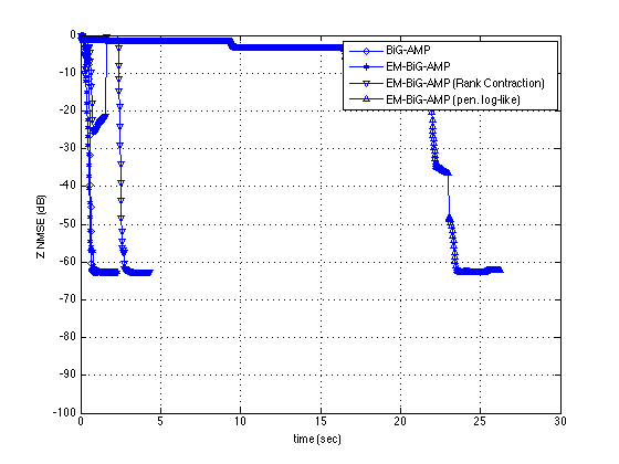
plotUtilityNew(results,[-100 0],200,201)

%Display the contents of the results structure
results{:}  %#ok<NOPTS>

ans = 

        name: 'BiG-AMP'
         err: -62.5967
        time: 1.7452
     errHist: [52x1 double]
    timeHist: [52x1 double]


ans = 

        name: 'EM-BiG-AMP'
         err: -62.5967
        time: 3.6378
     errHist: [122x1 double]
    timeHist: [122x1 double]


ans = 

        name: 'EM-BiG-AMP (Rank Contraction)'
         err: -62.5967
        time: 6.2815
     errHist: [204x1 double]
    timeHist: [204x1 double]
        rank: 4


ans = 

        name: 'EM-BiG-AMP (pen. log-like)'
         err: -62.5964
        time: 40.5503
     errHist: [1303x1 double]
    timeHist: [1303x1 double]
        rank: 4

Published with MATLAB® 7.14